1D Transient Transport, Initial Condition
The PFLOTRAN Input File (SUBSURFACE_TRANSPORT Mode)
The Problem Description
This problem is adapted from Faure, G. (1991), Principles and Applications of Inorganic Chemistry: A Comprehensive Textbook for Geology Students. New York: Macmillan Pub.Co., Section 19.3, pg.395, “Transport of Matter: Diffusion (Fick’s Second Law).”
The domain is a 1D column extending along the positive x-axis and is made up of 35x1x1 cubic grid cells with a length of 20 meters. The material is assigned the following properties: porosity = 1.0; tortuosity = 1.0; diffusion coefficient = 1.0e9 m2/s; which are homogenous in the domain.
The initial concentration of a generic tracer is assigned to 1.0e-20 (a value that is essentially zero but purposefully not exactly zero) everywhere, except at the center cell, where it is assigned a concentration of 20 Molar (mol/L). This initial pulse of tracer will diffuse over time, spreading itself out in both directions.
In PFLOTRAN, the initial concentration pulse in the center cell is homogeneous within that cell. However, the analytical solution describing the solution to Fick’s Second Law for an initial concentration pulse resembles a Dirac Delta function, which has an infinite value over a miniscule width. As the resolution of the grid increases, the initial condition on the PFLOTRAN grid will approach the Dirac Delta, but practically this limit cannot be reached. Therefore, for early times in the simulation, when the Dirac Delta pulse is beginning to relax, the PFLOTRAN solution will not match the analytical solution very well. However, the total amount of solute is the same, which can be verified by taking the integral of the concentration curve (ie, area under the solution curve).
The simulation is run for 80 years. The solution is plotted and compared at 10, 20, 40, and 80 years.
Fick’s Second Law governs the evolving tracer concentration,
The solution is given by,
where \(D\) is the diffusion coefficient, and \(c_0\) is the initial tracer concentration.
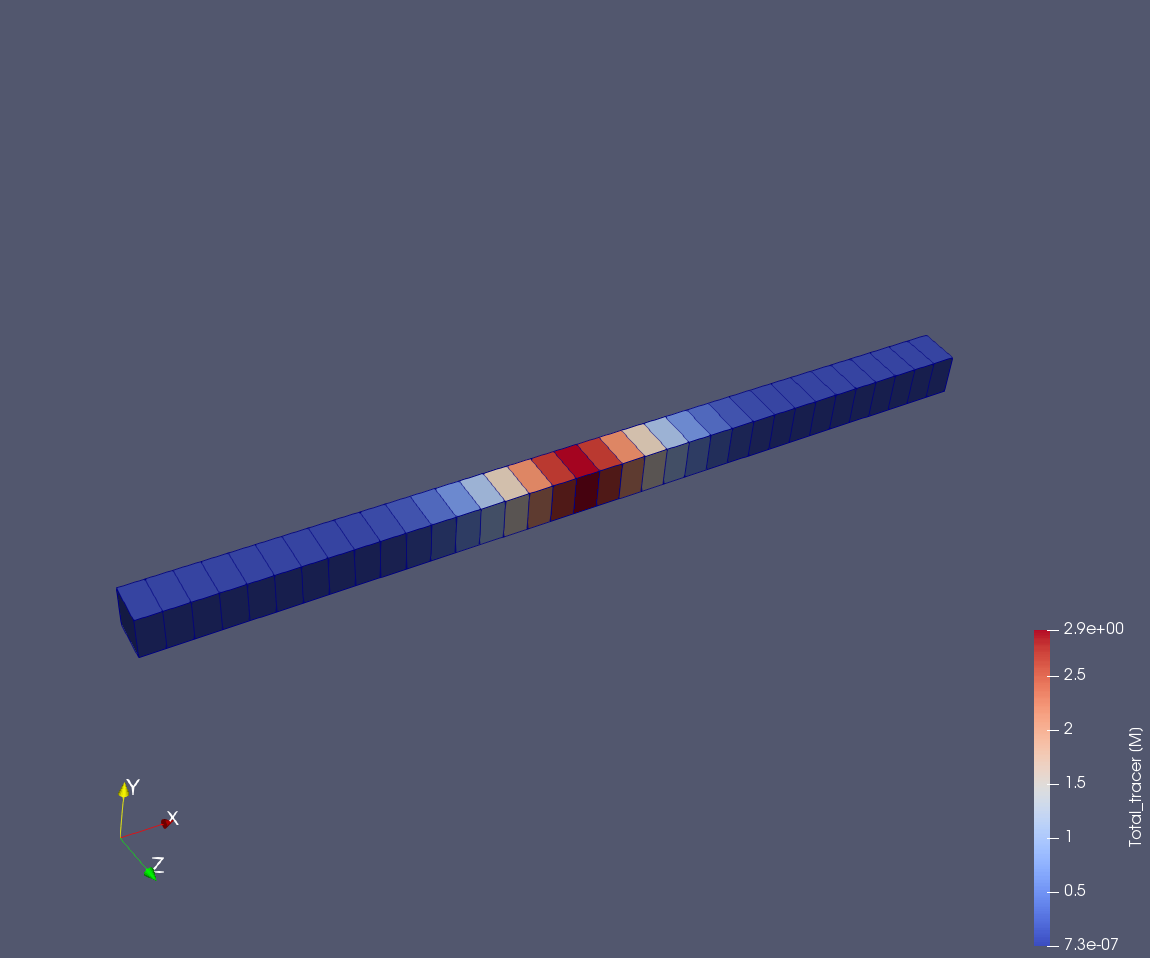
The PFLOTRAN domain set-up.
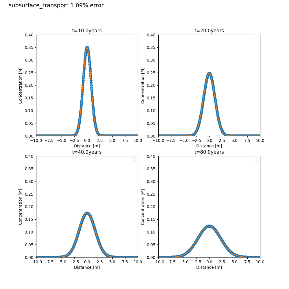
Comparison of the PFLOTRAN vs. analytical solution for SUBSURFACE_TRANSPORT mode.
The PFLOTRAN Input File (SUBSURFACE_TRANSPORT Mode)
The SUBSURFACE_TRANSPORT Mode PFLOTRAN input file can be downloaded
here.
SIMULATION
  SIMULATION_TYPE SUBSURFACE
  PROCESS_MODELS
    SUBSURFACE_TRANSPORT transport
      MODE GIRT
    /
  /
END

SUBSURFACE

CHEMISTRY
  PRIMARY_SPECIES
    tracer
  /
  #LOG_FORMULATION
  OUTPUT
    TOTAL
    ALL
  /
END

NUMERICAL_METHODS TRANSPORT
  LINEAR_SOLVER
    SOLVER DIRECT
  /
END

GRID
  TYPE structured
  NXYZ 575 1 1
  DXYZ
   0.034782608695652174d0
   1.0d0
   1.0d0
  END
END

REGION all
  COORDINATES
    0.0d0 0.0d0 0.0d0
    20.0d0 1.0d0 1.0d0
  /
END

REGION first_cell
  COORDINATES
    0.d0 0.d0 0.d0
    0.d0 1.d0 1.d0
  /
END

REGION middle_cell
  COORDINATES
    9.982608695652173d0 0.0d0 0.0d0
    10.017391304347827d0 1.0d0 1.0d0
  /
END


MATERIAL_PROPERTY soil1
  ID 1
  POROSITY 1.d0
  TORTUOSITY 1.d0
END

FLUID_PROPERTY
  DIFFUSION_COEFFICIENT 1.d-9
END

STRATA
  REGION all
  MATERIAL soil1
END

TIME
  FINAL_TIME 80.d0 y
  INITIAL_TIMESTEP_SIZE 1.d0 h
  MAXIMUM_TIMESTEP_SIZE 1.d-1 yr
END

OUTPUT
  SNAPSHOT_FILE
    TIMES y 10. 20. 40. 80.
    FORMAT HDF5
  /
END

TRANSPORT_CONDITION initial
  TYPE DIRICHLET
  CONSTRAINT_LIST
    0.d0 initial
  /
END

TRANSPORT_CONDITION initial_conc
  TYPE DIRICHLET
  CONSTRAINT_LIST
    0.d0 initial_conc
  /
END

INITIAL_CONDITION initial
  REGION all
  TRANSPORT_CONDITION initial
END

INITIAL_CONDITION intial_conc
  REGION middle_cell
  TRANSPORT_CONDITION initial_conc
END


CONSTRAINT initial_conc
  CONCENTRATIONS
    tracer 20.d0      T
  /
END

CONSTRAINT initial
  CONCENTRATIONS
    tracer 1.d-20     T
  /
END

END_SUBSURFACE
The Python Script
def transport_transient_1D_IC(path,input_prefix,remove,screen_on,pf_exe,mpi_exe,
                                                                      num_tries):
#==============================================================================#
# Based on:
# Faure, G.(1991). Principles and Applications of Inorganic Geochemistry:
# A Comprehensive Textbook for Geology Students. New York: Macmillan Pub.Co.
# Section 19.3, pg.395
# "TRANSPORT OF MATTER: DIFFUSION" (Fick's Second Law)
#
# Fick's Second Law (Eqn. 19.63)
# c = (pi * D * t)**-0.5 * e**(- x**2 / (4 * D * t)) * c_i
#
#    where,
#
#        t is time
#        x is distance
#        c is solute concentration at a given time
#        D is diffusion coefficient
#      c_i is initial solute concentration
#
# Date: 02/13/18
#*******************************************************************************
  nxyz = np.zeros(3) + 1
  dxyz = np.zeros(3) + 1.
  lxyz = np.zeros(3) + 1.
  error_analysis = np.zeros(num_tries)
  dxyz_record = np.zeros((num_tries,3))
  nxyz_record = np.zeros((num_tries,3))
  test_pass = False
  try_count = 0

  # Initial Discretization
  # Start refined enough that default NUM_TRIES=3 reaches <2% max relative error
  # (pure diffusion; coarser starts need 5+ doublings to pass the 2% criterion).
  lxyz[0] = 20.      # [m] lx
  nxyz[0] = 143      # [-] nx --> must start with odd number
  dxyz = lxyz/nxyz   # [m]
  pi = math.pi       # constant
  D = 1.0e-9         # [m^2/sec]
  c_i = 20.          # [M] concentration

  while (not test_pass) and (try_count < num_tries):
    print_discretization(lxyz,nxyz,dxyz)
    nx = int(nxyz[0]); ny = int(nxyz[1]); nz = int(nxyz[2])
    dx = dxyz[0]; dy = dxyz[1]; dz = dxyz[2]
    Lx = lxyz[0]; Ly = lxyz[1]; Lz = lxyz[2]
    try_count = try_count + 1

    x_soln = np.linspace(0.+(dx/2.),Lx-(dx/2.),nx) - Lx/2.  # [m]
    x_pflotran = np.linspace(0.+(dx/2.),Lx-(dx/2.),nx)      # [m]
    t_soln = np.array([10.,20.,40.,80.])                    # [y]
    c_soln = np.zeros((4,nx))                               # [M]
    c_pflotran = np.zeros((4,nx))                           # [M]

    vol = dx*dy*dz
    #print('cell volume = ' + str(vol) + ' m3')

    # create the analytical solution
    for time in range(4):
      t = t_soln[time]*365.0*24.0*3600.0     # [years -> sec]
      c_soln[time,:] = \
               (vol*c_i)*pow((4*pi*D*t),-0.5)*np.exp(-pow(x_soln,2.)/(4.*D*t))

    # run PFLOTRAN simulation
    run_pflotran(input_prefix,nxyz,dxyz,lxyz,remove,screen_on,pf_exe,mpi_exe)

    index_string = 'Time:  1.00000E+01 y/Total_tracer [M]'
    c_pflotran[0,:] = read_pflotran_output_1D(path+
                '/transient_1D_IC_subsurface_transport.h5',index_string,False)
    index_string = 'Time:  2.00000E+01 y/Total_tracer [M]'
    c_pflotran[1,:] = read_pflotran_output_1D(path+
                '/transient_1D_IC_subsurface_transport.h5',index_string,False)
    index_string = 'Time:  4.00000E+01 y/Total_tracer [M]'
    c_pflotran[2,:] = read_pflotran_output_1D(path+
                '/transient_1D_IC_subsurface_transport.h5',index_string,False)
    index_string = 'Time:  8.00000E+01 y/Total_tracer [M]'
    c_pflotran[3,:] = read_pflotran_output_1D(path+
                '/transient_1D_IC_subsurface_transport.h5',index_string,remove)
    ierr = check(c_pflotran)

    for g in range(4):
      area_soln = 0.
      area_p_soln = 0.
      for k in range(nx):
        area_soln = area_soln + c_soln[g,k]*dx
        area_p_soln = area_p_soln + c_pflotran[g,k]*dx
      #print('t='+str(g)+' analytical soln area = ' + str(area_soln) )
      #print('t='+str(g)+'   pflotran soln area = ' + str(area_p_soln) )

    max_percent_error = calc_relative_error(c_soln,c_pflotran,ierr)
    record_error(error_analysis,nxyz_record,dxyz_record,max_percent_error,
                 nxyz,dxyz,try_count)
    test_pass = does_pass(max_percent_error,try_count,num_tries)
    nxyz[0] = nxyz[0]*2.
    # ensure only odd number of cells
    if (nxyz[0]%2 == 0):
      nxyz[0] = nxyz[0] + 1
    dxyz = lxyz/nxyz

  # Plot the PFLOTRAN and analytical solutions
  plot_1D_transient(path,t_soln,'years',x_soln,c_soln,
                    x_soln,c_pflotran,'Distance [m]',
                    'Concentration [M]',"{0:.2f}".format(max_percent_error))
  # Plot error analysis
  plot_error(error_analysis,nxyz_record,dxyz_record,path,try_count,1)

  # Add test result to report card
  add_to_report(path,test_pass,max_percent_error,ierr)

  return;
Refer to section Python Helper Functions for documentation on the
qa_tests_helper module, which defines the helper functions used in the
Python script above.
