1D Steady Gas (Pressure), BCs of 1st Kind

The Problem Description

The PFLOTRAN Input File (GENERAL Mode)

The Python Script

The Problem Description

This problem is adapted from Kolditz, et al. (2015), Thermo-Hydro-Mechanical-Chemical Processes in Fractured Porous Media: Modelling and Benchmarking, Closed Form Solutions, Springer International Publishing, Switzerland. Section 2.3.1, pg.40, “A 1D Steady-State Gas Pressure Distribution, Boundary Conditions of 1st Kind.”

The domain is a 40x5x5 meter rectangular beam extending along the positive x-axis and is made up of 40x1x1 cubic grid cells with dimensions 1x5x5 meters. The materials are assigned the following properties: porosity = 0.5; gas viscosity \(\mu\) = 1.0e-5 Pa-s; permeability = 1e-15 m^2; gas saturation \(S_g\) = 1.0 in the entire domain.

The gas pressure is initially uniform at p(t=0) = 1.5e5 Pa. The boundary gas pressures are p(x=0) = 2.0e5 Pa and p(x=L) = 1.0e5 Pa, where L = 40 m. The simulation is run until the steady-state pressure distribution develops.

The LaPlace equation governs the steady-state gas pressure distribution,

\[{{\partial^{2} p^{2}} \over {\partial x^{2}}} = 0\]

The solution is given by,

\[p(x) = \sqrt{ax + b}\]

When the gas pressure boundary conditions are applied, the solution becomes,

\[p(x) = \sqrt{\left({p_1^2 - p_0^2}\right) {x \over L} + p_0^2}\]

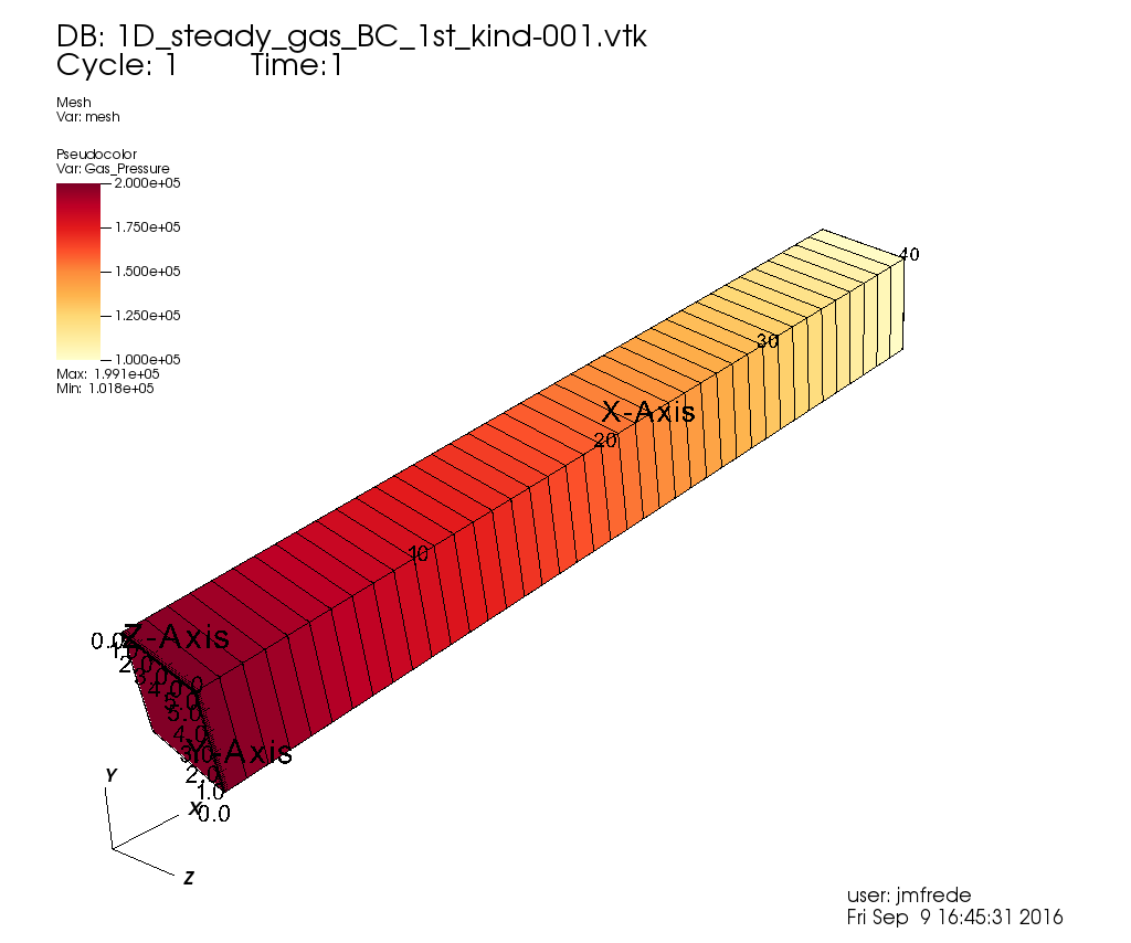
The PFLOTRAN domain set-up.

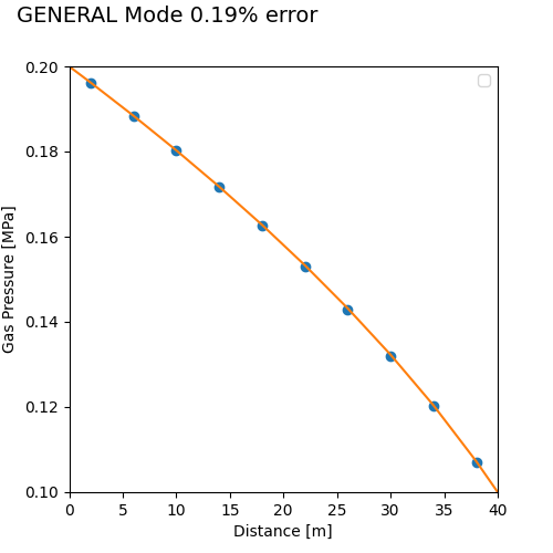
Comparison of the PFLOTRAN vs. analytical solution for GENERAL mode.

The PFLOTRAN Input File (GENERAL Mode)

The GENERAL Mode PFLOTRAN input file can be downloaded here.

 
SIMULATION
  SIMULATION_TYPE SUBSURFACE
  PROCESS_MODELS
    SUBSURFACE_FLOW flow
      MODE GENERAL
    /
  /
END

SUBSURFACE

GRID
  TYPE structured
  NXYZ 10 1 1
  DXYZ
   4.0d0
   1.0d0
   1.0d0
  END
END

REGION all
  COORDINATES
    0.0d0 0.0d0 0.0d0
    40.0d0 1.0d0 1.0d0
  /
END

REGION left_end
  FACE WEST
  COORDINATES
    0.d0 0.d0 0.d0
    0.d0 1.0d0 1.0d0
  /
END

REGION right_end
  FACE EAST
  COORDINATES
    40.0d0 0.d0 0.d0
    40.0d0 1.0d0 1.0d0
  /
END

MATERIAL_PROPERTY beam
  ID 1
  POROSITY 0.50
  TORTUOSITY 1.d0
  ROCK_DENSITY 2.8E3
  HEAT_CAPACITY 100.
  THERMAL_CONDUCTIVITY_DRY 1 W/m-C
  THERMAL_CONDUCTIVITY_WET 1 W/m-C
  CHARACTERISTIC_CURVES cc1
  PERMEABILITY
    PERM_X 1.d-15
    PERM_Y 1.d-15
    PERM_Z 1.d-15
  /
END

CHARACTERISTIC_CURVES cc1
  SATURATION_FUNCTION VAN_GENUCHTEN
    LIQUID_RESIDUAL_SATURATION 0.5d-1
    M 0.75
    ALPHA 1.d-3
  /
  PERMEABILITY_FUNCTION MUALEM
    LIQUID_RESIDUAL_SATURATION 0.05d0
    M 0.5d0
  /
  PERMEABILITY_FUNCTION MUALEM_VG_GAS
    LIQUID_RESIDUAL_SATURATION 0.05d0
    GAS_RESIDUAL_SATURATION 0.1d0
    M 0.5d0
  /
END

STRATA
  REGION all
  MATERIAL beam
END

EOS GAS
 VISCOSITY CONSTANT 1.0d-5 Pa-s
 #DENSITY CONSTANT 1.0 kg/m^3
END

FLUID_PROPERTY
  DIFFUSION_COEFFICIENT 1.d-9
END

TIME
  FINAL_TIME 1 yr
  INITIAL_TIMESTEP_SIZE 1.d-4 day
  MAXIMUM_TIMESTEP_SIZE 0.1d0 yr at 0.d0 yr
END

OUTPUT
  SNAPSHOT_FILE
    NO_PRINT_INITIAL
    #NO_PRINT_FINAL
    FORMAT HDF5
  /
END

FLOW_CONDITION initial
  TYPE
    TEMPERATURE dirichlet
    GAS_SATURATION dirichlet
    GAS_PRESSURE dirichlet
  /
  TEMPERATURE 25.d0 C
  GAS_SATURATION 1.0
  GAS_PRESSURE 1.5d5 Pa
END

FLOW_CONDITION left_end
  TYPE
    TEMPERATURE dirichlet
    GAS_SATURATION dirichlet
    GAS_PRESSURE dirichlet
  /
  TEMPERATURE 25.d0 C
  GAS_SATURATION 1.0
  GAS_PRESSURE 2.0d5 Pa
END

FLOW_CONDITION right_end
  TYPE
    TEMPERATURE dirichlet
    GAS_SATURATION dirichlet
    GAS_PRESSURE dirichlet
  /
  TEMPERATURE 25.d0 C
  GAS_SATURATION 1.0
  GAS_PRESSURE 1.0d5 Pa
END

INITIAL_CONDITION initial
  REGION all
  FLOW_CONDITION initial
END

BOUNDARY_CONDITION left_end
  REGION left_end
  FLOW_CONDITION left_end
END

BOUNDARY_CONDITION right_end
  FLOW_CONDITION right_end
  REGION right_end
END

END_SUBSURFACE

The Python Script

def gas_steady_1D_BC1stkind(path,input_prefix,remove,screen_on,pf_exe,
                                                             mpi_exe,num_tries):
#==============================================================================#
#
# Kolditz, et al. (2015) Thermo-Hydro-Mechanical-Chemical Processes in
# Fractured Porous Media: Modelling and Benchmarking, Closed Form Solutions,
# Springer International Publishing, Switzerland.
# Section 2.3.1, pg.40
# "A 1D Steady-State Gas Pressure Distribution, Boundary Conditions of 1st Kind"
#
# Author: Jenn Frederick
# Date: 09/09/2016
#*******************************************************************************
  nxyz = np.zeros(3) + 1
  dxyz = np.zeros(3) + 1.
  lxyz = np.zeros(3) + 1.
  error_analysis = np.zeros(num_tries)
  dxyz_record = np.zeros((num_tries,3))
  nxyz_record = np.zeros((num_tries,3))
  test_pass = False
  try_count = 0
  
  # initial discretization values
  lxyz[0] = 40.     # [m] lx
  nxyz[0] = 10      # [m] nx 
  dxyz = lxyz/nxyz  # [m]
  p0 = 2.0e5        # [Pa]
  p1 = 1.0e5        # [Pa]
  ierr = 0
  
  while (not test_pass) and (try_count < num_tries): 
    print_discretization(lxyz,nxyz,dxyz)
    nx = int(nxyz[0]); ny = int(nxyz[1]); nz = int(nxyz[2])
    dx = dxyz[0]; dy = dxyz[1]; dz = dxyz[2]
    Lx = lxyz[0]; Ly = lxyz[1]; Lz = lxyz[2]
    try_count = try_count + 1

    x_soln = np.linspace(0.+(dx/2.),Lx-(dx/2.),nx)  # [m]
    x_pflotran = x_soln                             # [m]
    x_soln = np.concatenate(([0.],x_soln),axis=0)   # [m]
    x_soln = np.concatenate((x_soln,[Lx]),axis=0)   # [m]
    p_soln = np.zeros(nx+2)                         # [Pa]
    p_pflotran = np.zeros(nx)                       # [Pa]

    # create the analytical solution
    p_soln = np.sqrt((((p1*p1) - (p0*p0))*(x_soln/Lx)) + (p0*p0)) # [Pa]
    
    # run PFLOTRAN simulation
    run_pflotran(input_prefix,nxyz,dxyz,lxyz,remove,screen_on,pf_exe,mpi_exe)
    
    # load data from hdf5
    index_string = 'Time:  1.00000E+00 y/Gas_Pressure [Pa]'
    p_pflotran[:] = read_pflotran_output_1D(path+
                    '/1D_steady_gas_BC_1st_kind.h5',index_string,remove)
    ierr = check(p_pflotran)

    # convert pressure units [Pa -> MPa]
    p_pflotran = p_pflotran/1.0e6         # [MPa]
    p_soln = p_soln/1.0e6                 # [MPa]

    max_percent_error = calc_relative_error(p_soln[1:nx+1],p_pflotran,ierr)
    record_error(error_analysis,nxyz_record,dxyz_record,max_percent_error,
                 nxyz,dxyz,try_count)
    test_pass = does_pass(max_percent_error,try_count,num_tries)
    nxyz[0] = nxyz[0]*2.
    dxyz = lxyz/nxyz

  # Plot the PFLOTRAN and analytical solutions
  plot_1D_steady(path,x_soln,p_soln,x_pflotran,p_pflotran,'Distance [m]',
                 'Gas Pressure [MPa]',"{0:.2f}".format(max_percent_error))
  
  # Plot error analysis
  plot_error(error_analysis,nxyz_record,dxyz_record,path,try_count,1)
  
  # Add test result to report card
  add_to_report(path,test_pass,max_percent_error,ierr)

  return;

Refer to section Python Helper Functions for documentation on the qa_tests_helper module, which defines the helper functions used in the Python script above.

1D Steady Gas (Pressure), BCs of 1st & 2nd Kind

The Problem Description

The PFLOTRAN Input File (GENERAL Mode)

The Python Script

The Problem Description

This problem is adapted from Kolditz, et al. (2015), Thermo-Hydro-Mechanical-Chemical Processes in Fractured Porous Media: Modelling and Benchmarking, Closed Form Solutions, Springer International Publishing, Switzerland. Section 2.3.2, pg.41, “A 1D Steady-State Gas Pressure Distribution, Boundary Conditions of 1st and 2nd Kind.”

The domain is a 40x5x5 meter rectangular beam extending along the positive x-axis and is made up of 40x1x1 cubic grid cells with dimensions 1x5x5 meters. The materials are assigned the following properties: porosity = 0.5; gas viscosity \(\mu\) = 1.0e-5 Pa-s; permeability = 1e-15 m^2; gas saturation \(S_g\) = 1.0 in the entire domain.

The gas pressure is initially uniform at p(t=0) = 1.0e5 Pa. At the east boundary, a dirichlet gas pressure p(x=L) = 1.0e5 Pa is applied, where L = 40 m. At the west boundary, a specific gas flow is applied Q(x=0) = 0.17 Pa m/s,

\[Q = -\frac{k}{\mu}p\frac{dp}{dx}\]

PFLOTRAN does not have the capability to handle such a boundary condition. To convert specific gas flow to a gas flux in m/s, the ideal gas law is used by dividing the specific gas flow by the boundary pressure,

\[p = \frac{n}{V}RT\]

where \(\frac{n}{V}\) is the gas density at the boundary in mol m^-1, R is the ideal gas constant (8.314), and T is the temperature in Kelvin. Therefore, the specific gas flow boundary at x=0 is converted to a gas flux boundary as,

(1)\[q = \frac{0.17}{\frac{n}{V}RT}\]

As gas flows into the domain, pressure increases, and as a result gas density also increases. To figure out what value of gas flux must be applied at the west boundary, we can use the analytical solution for gas pressure at x=0. Assuming a certain temperature, the gas density can be calculated using the ideal gas law. That gas density can then be used in equation (1) to set the value of the gas flux boundary condition. In this example, the gas pressure at steady state at the west boundary is approximately 4.4358 kg m^-3, which is converted to approximately 153.17 mol m^-3, giving \(\frac{n}{V}\). The values for R and T are known.

The simulation is run until the steady-state pressure distribution develops, which is 20 years.

The LaPlace equation governs the steady-state gas pressure distribution,

\[{{\partial^{2} p^{2}} \over {\partial x^{2}}} = 0\]

The solution is given by,

\[p(x) = \sqrt{ax + b}\]

When the boundary conditions are applied, the solution becomes,

\[p(x) = \sqrt{\frac{2 Q \mu}{k}(L-x) + p_1^2}\]

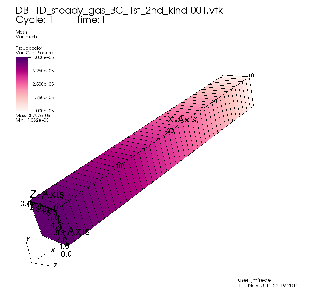
The PFLOTRAN domain set-up.

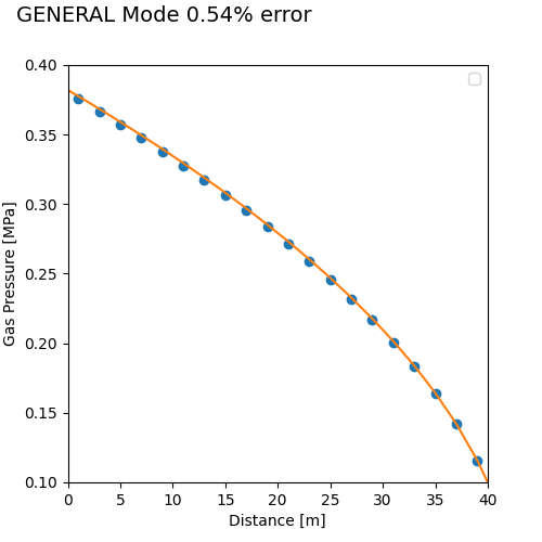
Comparison of the PFLOTRAN vs. analytical solution for GENERAL mode.

The PFLOTRAN Input File (GENERAL Mode)

The GENERAL Mode PFLOTRAN input file can be downloaded here.

 
SIMULATION
  SIMULATION_TYPE SUBSURFACE
  PROCESS_MODELS
    SUBSURFACE_FLOW flow
      MODE GENERAL
    /
  /
END

SUBSURFACE

GRID
  TYPE structured
  NXYZ 20 1 1
  DXYZ
   2.0d0
   1.0d0
   1.0d0
  END
END

REGION all
  COORDINATES
    0.0d0 0.0d0 0.0d0
    40.0d0 1.0d0 1.0d0
  /
END

REGION left_end
  FACE WEST
  COORDINATES
    0.d0 0.d0 0.d0
    0.d0 1.0d0 1.0d0
  /
END

REGION right_end
  FACE EAST
  COORDINATES
    40.0d0 0.d0 0.d0
    40.0d0 1.0d0 1.0d0
  /
END

REGION left_grid_cell
  COORDINATE 1.0d0 0.5d0 0.5d0 
END

MATERIAL_PROPERTY beam
  ID 1
  POROSITY 0.50
  TORTUOSITY 1.d0
  ROCK_DENSITY 2.8E3
  HEAT_CAPACITY 100.
  THERMAL_CONDUCTIVITY_DRY 1 W/m-C
  THERMAL_CONDUCTIVITY_WET 1 W/m-C
  CHARACTERISTIC_CURVES cc1
  PERMEABILITY
    PERM_X 1.d-15
    PERM_Y 1.d-15
    PERM_Z 1.d-15
  /
END

CHARACTERISTIC_CURVES cc1
  SATURATION_FUNCTION VAN_GENUCHTEN
    LIQUID_RESIDUAL_SATURATION 0.5d-1
    M 0.75
    ALPHA 1.d-3
  /
  PERMEABILITY_FUNCTION MUALEM
    LIQUID_RESIDUAL_SATURATION 0.05d0
    M 0.5d0
  /
  PERMEABILITY_FUNCTION MUALEM_VG_GAS
    LIQUID_RESIDUAL_SATURATION 0.05d0
    GAS_RESIDUAL_SATURATION 0.1d0
    M 0.5d0
  /
END

STRATA
  REGION all
  MATERIAL beam
END

EOS GAS
 VISCOSITY CONSTANT 1.0d-5 Pa-s
END

FLUID_PROPERTY
  DIFFUSION_COEFFICIENT 1.d-9
END

TIME
  FINAL_TIME 20 yr
  INITIAL_TIMESTEP_SIZE 1.d-4 day
  MAXIMUM_TIMESTEP_SIZE 0.01d0 yr at 0.d0 yr
END

OBSERVATION
  REGION left_grid_cell
END

OUTPUT
  SNAPSHOT_FILE
    NO_PRINT_INITIAL
    #NO_PRINT_FINAL
    FORMAT HDF5
  /
END

FLOW_CONDITION initial
  TYPE
    TEMPERATURE dirichlet
    MOLE_FRACTION dirichlet
    GAS_PRESSURE dirichlet
  /
  TEMPERATURE 25.d0 C
  MOLE_FRACTION 0.98
  GAS_PRESSURE 1.0d5 Pa
END

FLOW_CONDITION left_end
  TYPE
    TEMPERATURE dirichlet
    LIQUID_FLUX neumann
    GAS_FLUX neumann
  /
  TEMPERATURE 25.d0 C
  LIQUID_FLUX 0.d0 m/s
  # 0.17/((n/V)*R*T) = 0.17/(153.17*8.314*298.15)
  GAS_FLUX 4.475d-7 m/s
END

FLOW_CONDITION right_end
  TYPE
    TEMPERATURE dirichlet
    MOLE_FRACTION dirichlet
    GAS_PRESSURE dirichlet
  /
  TEMPERATURE 25.d0 C
  MOLE_FRACTION 0.98
  GAS_PRESSURE 1.0d5 Pa
END

INITIAL_CONDITION initial
  REGION all
  FLOW_CONDITION initial
END

BOUNDARY_CONDITION left_end
  REGION left_end
  FLOW_CONDITION left_end
END

BOUNDARY_CONDITION right_end
  FLOW_CONDITION right_end
  REGION right_end
END

END_SUBSURFACE

The Python Script

def gas_steady_1D_BC1st2ndkind(path,input_prefix,remove,screen_on,pf_exe,
                                                             mpi_exe,num_tries):
#==============================================================================#
#
# Kolditz, et al. (2015) Thermo-Hydro-Mechanical-Chemical Processes in
# Fractured Porous Media: Modelling and Benchmarking, Closed Form Solutions,
# Springer International Publishing, Switzerland.
# Section 2.3.2, pg.41
# "A 1D Steady-State Gas Pressure Distribution, Boundary Conditions of 1st 
# and 2nd Kind"
#
# Author: Jenn Frederick
# Date: 11/03/2016
#*******************************************************************************
  nxyz = np.zeros(3) + 1
  dxyz = np.zeros(3) + 1.
  lxyz = np.zeros(3) + 1.
  error_analysis = np.zeros(num_tries)
  dxyz_record = np.zeros((num_tries,3))
  nxyz_record = np.zeros((num_tries,3))
  test_pass = False
  try_count = 0
  
  # initial discretization values
  lxyz[0] = 40.     # [m] lx
  nxyz[0] = 20      # [m] nx 
  dxyz = lxyz/nxyz  # [m]
  k = 1.0e-15    # [m^2]
  mu = 1.0e-5    # [Pa*s]
  p1 = 1.0e5     # [Pa]
  Q = 0.17       # [Pa*m/s]
  ierr = 0
  
  while (not test_pass) and (try_count < num_tries): 
    print_discretization(lxyz,nxyz,dxyz)
    nx = int(nxyz[0]); ny = int(nxyz[1]); nz = int(nxyz[2])
    dx = dxyz[0]; dy = dxyz[1]; dz = dxyz[2]
    Lx = lxyz[0]; Ly = lxyz[1]; Lz = lxyz[2]
    try_count = try_count + 1

    x_soln = np.linspace(0.+(dx/2.),Lx-(dx/2.),nx)    # [m]
    x_pflotran = x_soln                               # [m]
    x_soln = np.concatenate(([0.],x_soln),axis=0)     # [m]
    x_soln = np.concatenate((x_soln,[Lx]),axis=0)     # [m]
    p_soln = np.zeros(nx+2)                           # [Pa]
    p_pflotran = np.zeros(nx)                         # [Pa]

    # create the analytical solution
    p_soln = np.sqrt(((2*Q*mu)/k)*(Lx-x_soln)+(p1**2)) # [Pa]

    # run PFLOTRAN simulation
    run_pflotran(input_prefix,nxyz,dxyz,lxyz,remove,screen_on,pf_exe,mpi_exe)

    # load data from hdf5
    index_string = 'Time:  2.00000E+01 y/Gas_Pressure [Pa]'
    p_pflotran[:] = read_pflotran_output_1D(path+
                    '/1D_steady_gas_BC_1st_2nd_kind.h5',index_string,remove)
    ierr = check(p_pflotran)

    # convert pressure units [Pa -> MPa]
    p_pflotran = p_pflotran/1.0e6         # [MPa]
    p_soln = p_soln/1.0e6                 # [MPa]

    max_percent_error = calc_relative_error(p_soln[1:nx+1],p_pflotran,ierr)
    record_error(error_analysis,nxyz_record,dxyz_record,max_percent_error,
                 nxyz,dxyz,try_count)
    test_pass = does_pass(max_percent_error,try_count,num_tries)
    nxyz[0] = nxyz[0]*2.
    dxyz = lxyz/nxyz

  # Plot the PFLOTRAN and analytical solutions
  plot_1D_steady(path,x_soln,p_soln,x_pflotran,p_pflotran,'Distance [m]',
                 'Gas Pressure [MPa]',"{0:.2f}".format(max_percent_error))
  
  # Plot error analysis
  plot_error(error_analysis,nxyz_record,dxyz_record,path,try_count,1)
  
  # Add test result to report card
  add_to_report(path,test_pass,max_percent_error,ierr)

  return;

Refer to section Python Helper Functions for documentation on the qa_tests_helper module, which defines the helper functions used in the Python script above.

2D Steady Gas (Pressure), BCs of 1st & 2nd Kind

The Problem Description

The PFLOTRAN Input File (GENERAL Mode)

The Dataset

The Python Script

The Problem Description

This problem is adapted from Kolditz, et al. (2015), Thermo-Hydro-Mechanical-Chemical Processes in Fractured Porous Media: Modelling and Benchmarking, Closed Form Solutions, Springer International Publishing, Switzerland. Section 2.3.3, pg.42, “A 2D Steady-State Gas Pressure Distribution, Boundary Conditions of 1st and 2nd Kind.”

The domain is a 1x1x0.5 meter rectangular plate extending along the positive x-axis and y-axis and is made up of 20x20x1 hexahedral grid cells with dimensions 0.05x0.05x0.5 meters. The materials are assigned the following properties: porosity = 0.5; gas viscosity \(\mu\) = 1.0e-5 Pa-s; permeability = 1e-15 m^2; gas saturation \(S_g\) = 1.0 in the entire domain.

The gas pressure is initially uniform at p(t=0) = 1.0e5 Pa. At the west and south boundaries, a dirichlet gas pressure p(x=0,y=(0,L)) = p(x=(0,L),y=0) = 1.0e5 Pa is applied, where L = 1 m. At the north and east boundaries, a specific gas flow [Pa m/s] is applied that is a function of x and y,

\[ \begin{align}\begin{aligned}Q = \frac{3 k p_0^2 y}{2 \mu L^2} \hspace{0.5 in} east \hspace{0.2 in} face\\Q = \frac{3 k p_0^2 x}{2 \mu L^2} \hspace{0.5 in} north \hspace{0.2 in} face\end{aligned}\end{align} \]

PFLOTRAN does not have the capability to handle such a boundary condition. For an explanation on how a specific gas flow is treated, see 1D Steady Gas (Pressure), BCs of 1st & 2nd Kind.

The simulation is run until the steady-state pressure distribution develops, which is 20 years.

The LaPlace equation governs the steady-state gas pressure distribution,

\[{{\partial^{2} p^{2}} \over {\partial x^{2}}} + {{\partial^{2} p^{2}} \over {\partial y^{2}}} = 0\]

When the boundary conditions are applied, the solution becomes,

\[p(x,y) = p_0 \sqrt{1 + 3\frac{xy}{L^2}}\]

where \(p_0\) is the initial pressure, p(t=0) = 1.0e5 Pa.

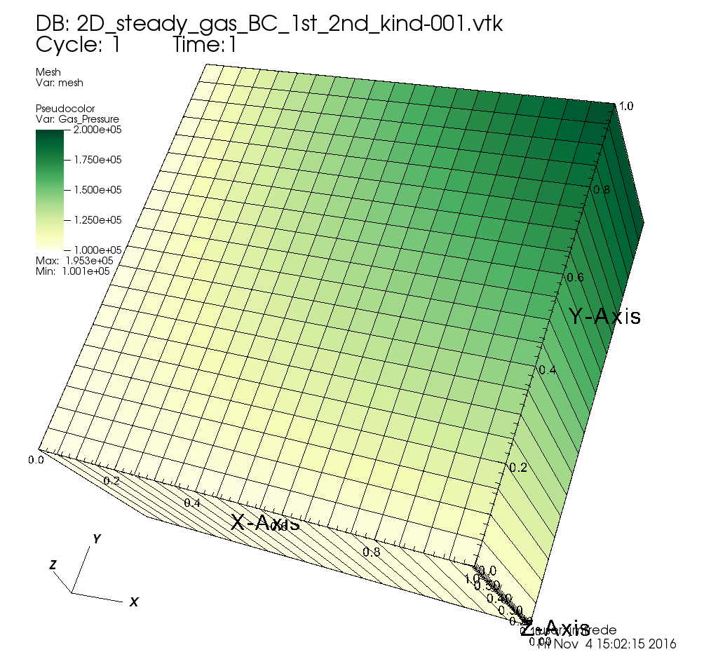
The PFLOTRAN domain set-up.

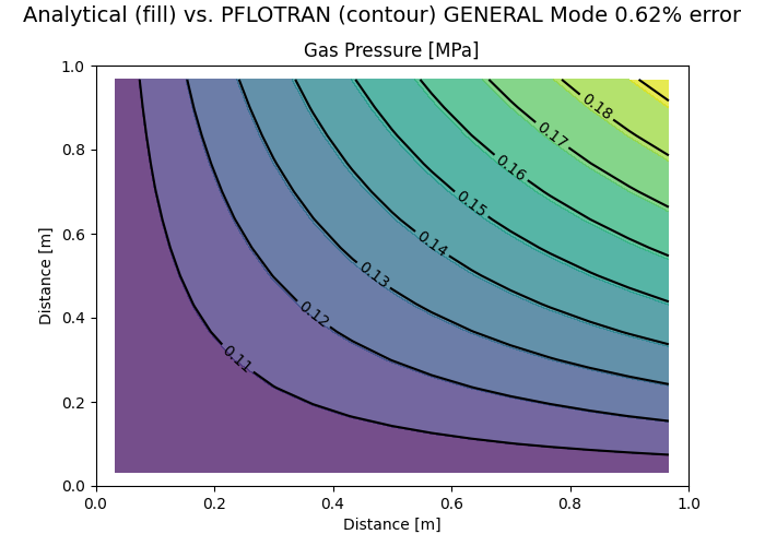
Comparison of the PFLOTRAN vs. analytical solution for GENERAL mode.

The PFLOTRAN Input File (GENERAL Mode)

The GENERAL Mode PFLOTRAN input file can be downloaded here.

 
SIMULATION
  SIMULATION_TYPE SUBSURFACE
  PROCESS_MODELS
    SUBSURFACE_FLOW flow
      MODE GENERAL
    /
  /
END

SUBSURFACE

GRID
  TYPE structured
  NXYZ 15 15 1
  DXYZ
   0.06666666666666667d0
   0.06666666666666667d0
   1.0d0
  END
END

REGION all
  COORDINATES
    0.0d0 0.0d0 0.0d0
    1.0d0 1.0d0 1.0d0
  /
END

REGION west_face
  FACE WEST
  COORDINATES
    0.d0 0.d0 0.d0
    0.d0 1.0d0 1.0d0
  /
END

REGION east_face
  FACE EAST
  COORDINATES
    1.0d0 0.d0 0.d0
    1.0d0 1.0d0 1.0d0
  /
END

REGION north_face
  FACE NORTH
  COORDINATES
    0.d0 1.0d0 0.d0
    1.0d0 1.0d0 1.0d0
  /
END

REGION south_face
  FACE SOUTH
  COORDINATES
    0.d0  0.d0  0.d0
    1.0d0 0.d0 1.0d0
  /
END

MATERIAL_PROPERTY plate
  ID 1
  POROSITY 0.50
  TORTUOSITY 1.d0
  ROCK_DENSITY 2.8E3
  HEAT_CAPACITY 100.
  THERMAL_CONDUCTIVITY_DRY 1 W/m-C
  THERMAL_CONDUCTIVITY_WET 1 W/m-C
  CHARACTERISTIC_CURVES cc1
  PERMEABILITY
    PERM_X 1.d-15
    PERM_Y 1.d-15
    PERM_Z 1.d-15
  /
END

CHARACTERISTIC_CURVES cc1
  SATURATION_FUNCTION VAN_GENUCHTEN
    LIQUID_RESIDUAL_SATURATION 0.5d-1
    M 0.75
    ALPHA 1.d-3
  /
  PERMEABILITY_FUNCTION MUALEM
    LIQUID_RESIDUAL_SATURATION 0.05d0
    M 0.5d0
  /
  PERMEABILITY_FUNCTION MUALEM_VG_GAS
    LIQUID_RESIDUAL_SATURATION 0.05d0
    GAS_RESIDUAL_SATURATION 0.1d0
    M 0.5d0
  /
END

STRATA
  REGION all
  MATERIAL plate
END

FLUID_PROPERTY
  DIFFUSION_COEFFICIENT 1.d-9
END

EOS GAS
 VISCOSITY CONSTANT 1.0d-5 Pa-s
END

TIME
  FINAL_TIME 10 yr
  INITIAL_TIMESTEP_SIZE 1.d-4 day
  MAXIMUM_TIMESTEP_SIZE 0.01d0 yr at 0.d0 yr
END

OUTPUT
  SNAPSHOT_FILE
    NO_PRINT_INITIAL
    #NO_PRINT_FINAL
    FORMAT HDF5
  /
END

DATASET flux_bc_north
  HDF5_DATASET_NAME x_line_cell_centered_north
  FILENAME ../dataset.h5
END

DATASET flux_bc_east
  HDF5_DATASET_NAME y_line_cell_centered_east
  FILENAME ../dataset.h5
END

FLOW_CONDITION initial
  TYPE
    TEMPERATURE dirichlet
    MOLE_FRACTION dirichlet
    GAS_PRESSURE dirichlet
  /
  TEMPERATURE 25.d0 C
  MOLE_FRACTION 0.98
  GAS_PRESSURE 1.0d5 Pa
END

FLOW_CONDITION east_face
  TYPE
    TEMPERATURE dirichlet
    LIQUID_FLUX neumann
    GAS_FLUX neumann
  /
  TEMPERATURE 25.d0 C
  LIQUID_FLUX 0.d0 m/s
  GAS_FLUX DATASET flux_bc_east
END

FLOW_CONDITION north_face
  TYPE
    TEMPERATURE dirichlet
    LIQUID_FLUX neumann
    GAS_FLUX neumann
  /
  TEMPERATURE 25.d0 C
  LIQUID_FLUX 0.d0 m/s
  GAS_FLUX DATASET flux_bc_north
END

FLOW_CONDITION dirichlet_pressure
  TYPE
    TEMPERATURE dirichlet
    MOLE_FRACTION dirichlet
    GAS_PRESSURE dirichlet
  /
  TEMPERATURE 25.d0 C
  MOLE_FRACTION 0.98
  GAS_PRESSURE 1.0d5 Pa
END

INITIAL_CONDITION initial
  REGION all
  FLOW_CONDITION initial
END

BOUNDARY_CONDITION west_face
  REGION west_face
  FLOW_CONDITION dirichlet_pressure
END

BOUNDARY_CONDITION south_face
  REGION south_face
  FLOW_CONDITION dirichlet_pressure
END

BOUNDARY_CONDITION east_face
  FLOW_CONDITION east_face
  REGION east_face
END

BOUNDARY_CONDITION north_face
  FLOW_CONDITION north_face
  REGION north_face
END

END_SUBSURFACE

The Dataset

The hdf5 dataset required to define the boundary conditions is created with the following python script called create_dataset.py:

import sys
from h5py import *
import numpy as np

nx = 1; dx = 1; lx = 1
ny = 1; dy = 1; ly = 1
nz = 1; dz = 1; lz = 1
for k in range(len(sys.argv)-1):
  k = k + 1
  if sys.argv[k] == '-nx':
    nx = int(float(sys.argv[k+1]))
  if sys.argv[k] == '-ny':
    ny = int(float(sys.argv[k+1]))
  if sys.argv[k] == '-nz':
    nz = int(float(sys.argv[k+1]))
  if sys.argv[k] == '-dx':
    dx = float(sys.argv[k+1])
  if sys.argv[k] == '-dy':
    dy = float(sys.argv[k+1])
  if sys.argv[k] == '-dz':
    dz = float(sys.argv[k+1])
  if sys.argv[k] == '-lx':
    lx = float(sys.argv[k+1])
  if sys.argv[k] == '-ly':
    ly = float(sys.argv[k+1])
  if sys.argv[k] == '-lz':
    lz = float(sys.argv[k+1])

filename = 'dataset.h5'
h5file = File(filename,mode='w')

p0 = 1.0e5   # [Pa]
k = 1.0e-15  # [m2]
mu = 1.0e-5  # [Pa-s]

# 1d line in x
# Flux boundary condition; NORTH
h5grp = h5file.create_group('x_line_cell_centered_north')
h5grp.attrs['Cell Centered'] = True
h5grp.attrs['Space Interpolation Method'] = np.bytes_('STEP')
h5grp.attrs['Dimension'] = np.bytes_('X')
# Delta length between points [m]
h5grp.attrs['Discretization'] = [dx]
# Location of origin
h5grp.attrs['Origin'] = [0.]
# Load the dataset values
rarray = np.zeros(nx,'=f8')
for i in range(nx):
  x = (float(i)*lx)/nx + dx/2.
  p_gas = p0*np.sqrt(1+3*(x/lx))  # [Pa] from analytical solution at y=L
  rarray[i] = ((3*k)/(2*mu))*((p0**2)/lx)*(x/lx)   # [Pa m/s]
  rarray[i] = rarray[i]/p_gas                      # [m/s]
h5dset = h5grp.create_dataset('Data', data=rarray)

# 1d line in y
# Flux boundary condition; EAST
h5grp = h5file.create_group('y_line_cell_centered_east')
h5grp.attrs['Cell Centered'] = True
h5grp.attrs['Space Interpolation Method'] = np.bytes_('STEP')
h5grp.attrs['Dimension'] = np.bytes_('Y')
# Delta length between points [m]
h5grp.attrs['Discretization'] = [dy]
# Location of origin
h5grp.attrs['Origin'] = [0.]
# Load the dataset values
rarray = np.zeros(ny,'=f8')
for i in range(ny):
  y = (float(i)*ly)/ny + dy/2.
  p_gas = p0*np.sqrt(1+3*(y/ly))  # [Pa] from analytical solution at x=L
  rarray[i] = ((3*k)/(2*mu))*((p0**2)/ly)*(y/ly)   # [Pa m/s]
  rarray[i] = rarray[i]/p_gas                      # [m/s]
h5dset = h5grp.create_dataset('Data', data=rarray)

The Python Script

def gas_steady_2D_BC1st2ndkind(path,input_prefix,remove,screen_on,pf_exe,
                                                             mpi_exe,num_tries):
#==============================================================================#
#
# Kolditz, et al. (2015) Thermo-Hydro-Mechanical-Chemical Processes in
# Fractured Porous Media: Modelling and Benchmarking, Closed Form Solutions,
# Springer International Publishing, Switzerland.
# Section 2.3.3, pg.42
# "A 2D Steady-State Gas Pressure Distribution, Boundary Conditions of 1st 
# and 2nd Kind"
#
# Author: Jenn Frederick
# Date: 11/04/2016
#*******************************************************************************
  nxyz = np.zeros(3) + 1
  dxyz = np.zeros(3) + 1.
  lxyz = np.zeros(3) + 1.
  error_analysis = np.zeros(num_tries)
  dxyz_record = np.zeros((num_tries,3))
  nxyz_record = np.zeros((num_tries,3))
  test_pass = False
  try_count = 0
  
  # initial discretization values
  lxyz[0] = 1.      # [m] lx
  lxyz[1] = 1.      # [m] ly
  nxyz[0] = 15      # [m] nx 
  nxyz[1] = 15      # [m] ny 
  dxyz = lxyz/nxyz  # [m]
  p0 = 1.0e5        # [Pa]
  ierr = 0
  
  while (not test_pass) and (try_count < num_tries): 
    print_discretization(lxyz,nxyz,dxyz)
    nx = int(nxyz[0]); ny = int(nxyz[1]); nz = int(nxyz[2])
    dx = dxyz[0]; dy = dxyz[1]; dz = dxyz[2]
    Lx = lxyz[0]; Ly = lxyz[1]; Lz = lxyz[2]
    try_count = try_count + 1

    p_soln = np.zeros((nx,ny))                       # [Pa]
    p_pflotran = np.zeros((nx,ny))                   # [Pa]
    x_soln = np.linspace(0.+(dx/2.),Lx-(dx/2.),nx)   # [m]
    y_soln = np.linspace(0.+(dy/2.),Ly-(dy/2.),ny)   # [m]

    # create the analytical solution
    i = -1
    for x in x_soln:
      i = i + 1
      j = -1
      for y in y_soln:
        j = j + 1
        p_soln[i,j] = p0*np.sqrt(1+3*((x*y)/(Lx*Ly)))

    # run PFLOTRAN simulation
    os.chdir('../')
    command_line = sys.executable + ' create_dataset.py'
    command_line = command_line + ' -nx ' + str(nx) + ' -ny ' + str(ny)
    command_line = command_line + ' -lx ' + str(Lx) + ' -ly ' + str(Ly)
    command_line = command_line + ' -dx ' + str(dx) + ' -dy ' + str(dy)
    os.system(command_line)
    os.chdir('general_mode')
    run_pflotran(input_prefix,nxyz,dxyz,lxyz,remove,screen_on,pf_exe,mpi_exe)

    # load data from hdf5
    index_string = 'Time:  1.00000E+01 y/Gas_Pressure [Pa]'
    p_pflotran[:,:] = read_pflotran_output_2D(path+
                      '/2D_steady_gas_BC_1st_2nd_kind.h5',index_string,remove)
    ierr = check(p_pflotran)

    # convert pressure units [Pa -> MPa]
    p_pflotran = p_pflotran/1.0e6         # [MPa]
    p_soln = p_soln/1.0e6                 # [MPa]

    max_percent_error = calc_relative_error(p_soln,p_pflotran,ierr)
    record_error(error_analysis,nxyz_record,dxyz_record,max_percent_error,
                 nxyz,dxyz,try_count)
    test_pass = does_pass(max_percent_error,try_count,num_tries)
    nxyz[0] = nxyz[0]*2.
    nxyz[1] = nxyz[1]*2.
    dxyz = lxyz/nxyz

  # Plot the PFLOTRAN and analytical solutions
  plot_2D_steady(path,x_soln,y_soln,p_soln,p_pflotran,'Distance [m]',
                 'Gas Pressure [MPa]',"{0:.2f}".format(max_percent_error))
  
  # Plot error analysis
  plot_error(error_analysis,nxyz_record,dxyz_record,path,try_count,2)
  
  # Add test result to report card
  add_to_report(path,test_pass,max_percent_error,ierr)

  return;

Refer to section Python Helper Functions for documentation on the qa_tests_helper module, which defines the helper functions used in the Python script above.

3D Steady Gas (Pressure), BCs of 2nd Kind

The Problem Description

The PFLOTRAN Input File (GENERAL Mode)

The Dataset

The Python Script

The Problem Description

This problem is adapted from Kolditz, et al. (2015), Thermo-Hydro-Mechanical-Chemical Processes in Fractured Porous Media: Modelling and Benchmarking, Closed Form Solutions, Springer International Publishing, Switzerland. Section 2.3.4, pg.43, “A 3D Steady-State Gas Pressure Distribution, Boundary Conditions of 2nd Kind.”

The domain is a 1x1x1 meter cube extending along the positive x-axis, y-axis, and z-axis and is made up of 20x20x20 hexahedral grid cells with dimensions 0.05x0.05x0.05 meters. The material is assigned the following properties: porosity = 0.5; gas viscosity \(\mu\) = 1.0e-5 Pa-s; permeability = 1e-15 m^2; gas saturation \(S_g\) = 1.0 in the entire domain.

The gas pressure is initially uniform at p(t=0) = 1.0e5 Pa. At each face of the cube, a specific gas flow [Pa m/s] boundary condition is applied:

\[ \begin{align}\begin{aligned}-Q(0,y,z) = Q(L,y,z) = \frac{3 k p_0^2 y}{4 \mu L^2}\\-Q(x,0,z) = Q(x,L,z) = \frac{3 k p_0^2 x}{4 \mu L^2}\\-Q(x,y,0) = Q(x,y,L) = \frac{3 k p_0^2 }{4 \mu L}\end{aligned}\end{align} \]

Note that this specific gas flow boundary condition acts as a source on the faces where x, y, or z = L, and a sink on the faces where x, y, or z = 0. PFLOTRAN does not have the capability to handle such a boundary condition. For an explanation on how a specific gas flow is treated, see 1D Steady Gas (Pressure), BCs of 1st & 2nd Kind.

The simulation is run until the steady-state pressure distribution develops, which is 10 years.

The LaPlace equation governs the steady-state gas pressure distribution,

\[{{\partial^{2} p^{2}} \over {\partial x^{2}}} + {{\partial^{2} p^{2}} \over {\partial y^{2}}} + {{\partial^{2} p^{2}} \over {\partial z^{2}}} = 0\]

When the boundary conditions are applied, the solution becomes,

\[p(x,y,z) = p_0 \sqrt{1 + \frac{3}{2}\left({\frac{xy}{L^2}+\frac{z}{L}}\right)}\]

where \(p_0\) is the initial pressure, p(t=0) = 1.0e5 Pa.

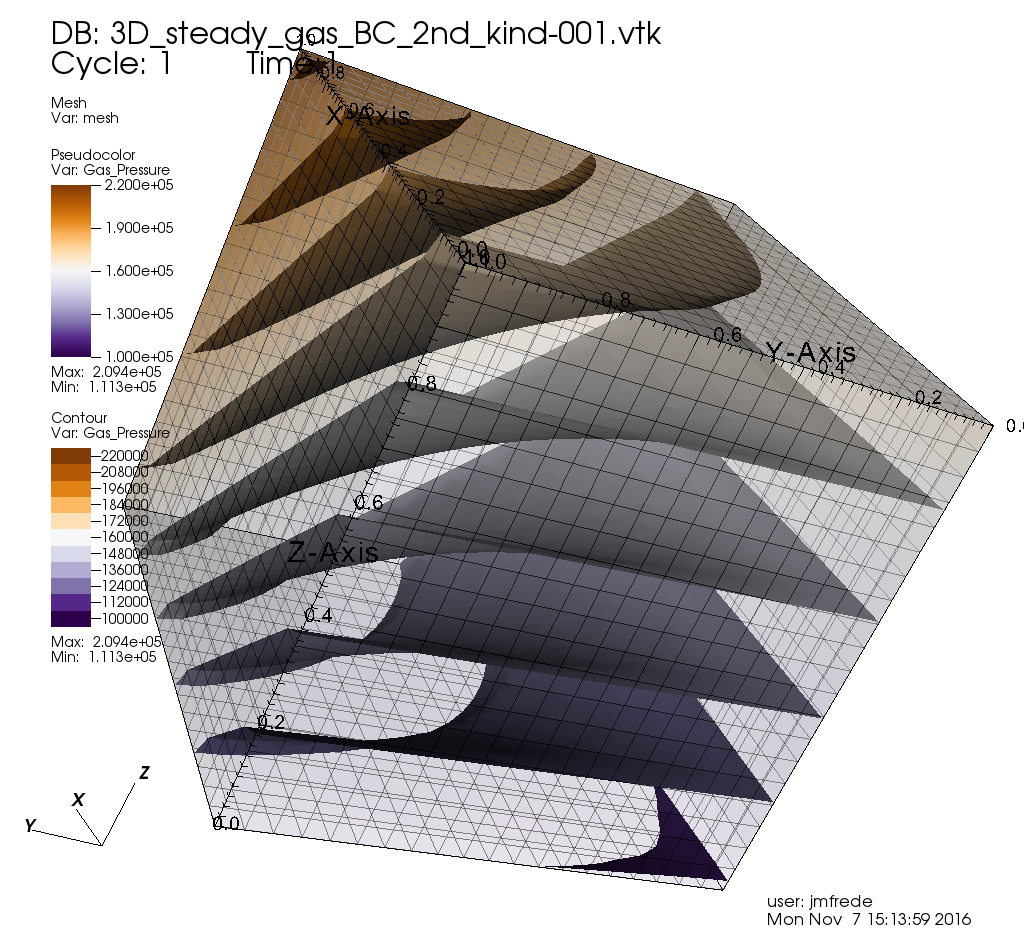
The PFLOTRAN domain set-up.

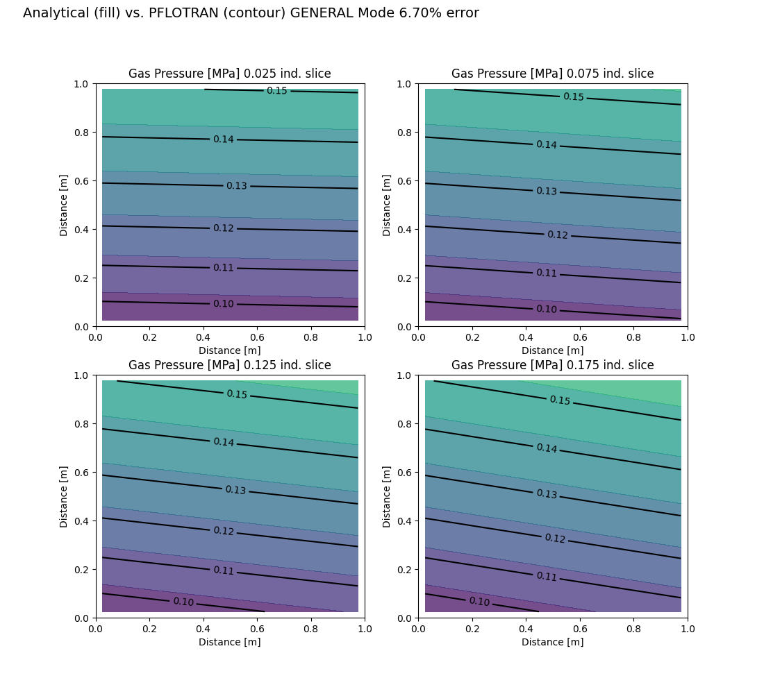
Comparison of the PFLOTRAN vs. analytical solution for GENERAL mode.

The PFLOTRAN Input File (GENERAL Mode)

The GENERAL Mode PFLOTRAN input file can be downloaded here.

 
SIMULATION
  SIMULATION_TYPE SUBSURFACE
  PROCESS_MODELS
    SUBSURFACE_FLOW flow
      MODE GENERAL
    /
  /
END

SUBSURFACE

GRID
  TYPE structured
  NXYZ 20 20 20
  DXYZ
   0.05d0
   0.05d0
   0.05d0
  END
END

REGION all
  COORDINATES
    0.0d0 0.0d0 0.0d0
    1.0d0 1.0d0 1.0d0
  /
END

REGION west_face
  FACE WEST
  COORDINATES
    0.d0 0.d0 0.d0
    0.d0 1.0d0 1.0d0
  /
END

REGION east_face
  FACE EAST
  COORDINATES
    1.0d0 0.d0 0.d0
    1.0d0 1.0d0 1.0d0
  /
END

REGION north_face
  FACE NORTH
  COORDINATES
    0.d0 1.0d0 0.d0
    1.0d0 1.0d0 1.0d0
  /
END

REGION south_face
  FACE SOUTH
  COORDINATES
    0.d0 0.d0 0.d0
    1.0d0 0.d0 1.0d0
  /
END

REGION bottom_face
  FACE BOTTOM
  COORDINATES
    0.d0 0.d0 0.d0
    1.0d0 1.0d0 0.d0
  /
END

REGION top_face
  FACE TOP
  COORDINATES
    0.d0 0.d0 1.0d0
    1.0d0 1.0d0 1.0d0
  /
END

MATERIAL_PROPERTY cube
  ID 1
  POROSITY 0.50
  TORTUOSITY 1.d0
  ROCK_DENSITY 2.8E3
  HEAT_CAPACITY 100.
  THERMAL_CONDUCTIVITY_DRY 1 W/m-C
  THERMAL_CONDUCTIVITY_WET 1 W/m-C
  CHARACTERISTIC_CURVES cc1
  PERMEABILITY
    PERM_X 1.d-15
    PERM_Y 1.d-15
    PERM_Z 1.d-15
  /
END

CHARACTERISTIC_CURVES cc1
  SATURATION_FUNCTION VAN_GENUCHTEN
    LIQUID_RESIDUAL_SATURATION 0.5d-1
    M 0.75
    ALPHA 1.d-3
  /
  PERMEABILITY_FUNCTION MUALEM
    LIQUID_RESIDUAL_SATURATION 0.05d0
    M 0.5d0
  /
  PERMEABILITY_FUNCTION MUALEM_VG_GAS
    LIQUID_RESIDUAL_SATURATION 0.05d0
    GAS_RESIDUAL_SATURATION 0.1d0
    M 0.5d0
  /
END

STRATA
  REGION all
  MATERIAL cube
END

FLUID_PROPERTY
  DIFFUSION_COEFFICIENT 1.d-9
END

EOS GAS
 VISCOSITY CONSTANT 1.0d-5 Pa-s
END

TIME
  FINAL_TIME 10 yr
  INITIAL_TIMESTEP_SIZE 1.d-4 day
  MAXIMUM_TIMESTEP_SIZE 0.01d0 yr at 0.d0 yr
END

OUTPUT
  SNAPSHOT_FILE
    NO_PRINT_INITIAL
    #NO_PRINT_FINAL
    FORMAT HDF5
  /
END

DATASET flux_bc_west
  HDF5_DATASET_NAME cell_centered_surf_west
  FILENAME ../dataset.h5
END

DATASET flux_bc_east
  HDF5_DATASET_NAME cell_centered_surf_east
  FILENAME ../dataset.h5
END

DATASET flux_bc_north
  HDF5_DATASET_NAME cell_centered_surf_north
  FILENAME ../dataset.h5
END

DATASET flux_bc_south
  HDF5_DATASET_NAME cell_centered_surf_south
  FILENAME ../dataset.h5
END

DATASET flux_bc_top
  HDF5_DATASET_NAME cell_centered_surf_top
  FILENAME ../dataset.h5
END

DATASET flux_bc_bottom
  HDF5_DATASET_NAME cell_centered_surf_bottom
  FILENAME ../dataset.h5
END

FLOW_CONDITION initial
  TYPE
    TEMPERATURE dirichlet
    MOLE_FRACTION dirichlet
    GAS_PRESSURE dirichlet
  /
  TEMPERATURE 25.d0 C
  MOLE_FRACTION 0.98
  GAS_PRESSURE 1.0d5 Pa
END

FLOW_CONDITION east_face
  TYPE
    TEMPERATURE dirichlet
    LIQUID_FLUX neumann
    GAS_FLUX neumann
  /
  TEMPERATURE 25.d0 C
  LIQUID_FLUX 0.d0 m/s
  GAS_FLUX DATASET flux_bc_east
END

FLOW_CONDITION west_face
  TYPE
    TEMPERATURE dirichlet
    LIQUID_FLUX neumann
    GAS_FLUX neumann
  /
  TEMPERATURE 25.d0 C
  LIQUID_FLUX 0.d0 m/s
  GAS_FLUX DATASET flux_bc_west
END

FLOW_CONDITION north_face
  TYPE
    TEMPERATURE dirichlet
    LIQUID_FLUX neumann
    GAS_FLUX neumann
  /
  TEMPERATURE 25.d0 C
  LIQUID_FLUX 0.d0 m/s
  GAS_FLUX DATASET flux_bc_north
END

FLOW_CONDITION south_face
  TYPE
    TEMPERATURE dirichlet
    LIQUID_FLUX neumann
    GAS_FLUX neumann
  /
  TEMPERATURE 25.d0 C
  LIQUID_FLUX 0.d0 m/s
  GAS_FLUX DATASET flux_bc_south
END

FLOW_CONDITION top_face
  TYPE
    TEMPERATURE dirichlet
    LIQUID_FLUX neumann
    GAS_FLUX neumann
  /
  TEMPERATURE 25.d0 C
  LIQUID_FLUX 0.d0 m/s
  GAS_FLUX DATASET flux_bc_top
END

FLOW_CONDITION bottom_face
  TYPE
    TEMPERATURE dirichlet
    LIQUID_FLUX neumann
    GAS_FLUX neumann
  /
  TEMPERATURE 25.d0 C
  LIQUID_FLUX 0.d0 m/s
  GAS_FLUX DATASET flux_bc_bottom
END

INITIAL_CONDITION initial
  REGION all
  FLOW_CONDITION initial
END

BOUNDARY_CONDITION west_face
  REGION west_face
  FLOW_CONDITION west_face
END

BOUNDARY_CONDITION east_face
  FLOW_CONDITION east_face
  REGION east_face
END

BOUNDARY_CONDITION north_face
  REGION north_face
  FLOW_CONDITION north_face
END

BOUNDARY_CONDITION south_face
  FLOW_CONDITION south_face
  REGION south_face
END

BOUNDARY_CONDITION bottom_face
  REGION bottom_face
  FLOW_CONDITION bottom_face
END

BOUNDARY_CONDITION top_face
  FLOW_CONDITION top_face
  REGION top_face
END

END_SUBSURFACE

The Dataset

The hdf5 dataset required to define the boundary conditions is created with the following python script called create_dataset.py:

import sys
from h5py import *
import numpy as np

nx = 1; dx = 1; lx = 1
ny = 1; dy = 1; ly = 1
nz = 1; dz = 1; lz = 1
for k in range(len(sys.argv)-1):
  k = k + 1
  if sys.argv[k] == '-nx':
    nx = int(float(sys.argv[k+1]))
  if sys.argv[k] == '-ny':
    ny = int(float(sys.argv[k+1]))
  if sys.argv[k] == '-nz':
    nz = int(float(sys.argv[k+1]))
  if sys.argv[k] == '-dx':
    dx = float(sys.argv[k+1])
  if sys.argv[k] == '-dy':
    dy = float(sys.argv[k+1])
  if sys.argv[k] == '-dz':
    dz = float(sys.argv[k+1])
  if sys.argv[k] == '-lx':
    lx = float(sys.argv[k+1])
  if sys.argv[k] == '-ly':
    ly = float(sys.argv[k+1])
  if sys.argv[k] == '-lz':
    lz = float(sys.argv[k+1])

filename = 'dataset.h5'
h5file = File(filename,mode='w')

p0 = 1.0e5   # [Pa]
K = 1.0e-15  # [m2]
mu = 1.0e-5  # [Pa-s]

# 2D Surface:
# -----------------------------------------------------------------------------
# Gas flux boundary condition x=0 face
h5grp = h5file.create_group('cell_centered_surf_west')
h5grp.attrs['Dimension'] = np.bytes_('YZ')
h5grp.attrs['Cell Centered'] = True
h5grp.attrs['Space Interpolation Method'] = np.bytes_('STEP')
# Delta length between points [m]
h5grp.attrs['Discretization'] = [dy,dz]
# Location of origin
h5grp.attrs['Origin'] = [0.,0.]
# Load the dataset values
rarray = np.zeros((ny,nz),'=f8')
for j in range(ny):
  for k in range(nz):
    x = 0.
    y = (float(j)*ly)/(ny) + dy/2.
    z = (float(k)*lz)/(nz) + dz/2.
    p_gas = p0*np.sqrt(1.+(3./2.)*((x/lx)*(y/ly)+(z/lz)))
    rarray[j][k] = ((3.*K)/(4.*mu))*(p0**2/lx)*(y/ly)
    # flow is out: (-)
    rarray[j][k] = -1.0*rarray[j][k]/p_gas
h5dset = h5grp.create_dataset('Data', data=rarray)

# 2D Surface:
# -----------------------------------------------------------------------------
# Gas flux boundary condition x=L face
h5grp = h5file.create_group('cell_centered_surf_east')
h5grp.attrs['Dimension'] = np.bytes_('YZ')
h5grp.attrs['Cell Centered'] = True
h5grp.attrs['Space Interpolation Method'] = np.bytes_('STEP')
# Delta length between points [m]
h5grp.attrs['Discretization'] = [dy,dz]
# Location of origin
h5grp.attrs['Origin'] = [0.,0.]
# Load the dataset values
rarray = np.zeros((ny,nz),'=f8')
for j in range(ny):
  for k in range(nz):
    x = lx
    y = (float(j)*ly)/(ny) + dy/2.
    z = (float(k)*lz)/(nz) + dz/2.
    p_gas = p0*np.sqrt(1+(3/2)*((x/lx)*(y/ly)+(z/lz)))  # [Pa] from analytical solution
    rarray[j][k] = ((3.*K)/(4.*mu))*(p0**2/lx)*(y/ly)   # [Pa m/s]
    rarray[j][k] = rarray[j][k]/p_gas                   # [m/s]
h5dset = h5grp.create_dataset('Data', data=rarray)

# 2D Surface:
# -----------------------------------------------------------------------------
# Gas flux boundary condition z=0 face
h5grp = h5file.create_group('cell_centered_surf_bottom')
h5grp.attrs['Dimension'] = np.bytes_('XY')
h5grp.attrs['Cell Centered'] = True
h5grp.attrs['Space Interpolation Method'] = np.bytes_('STEP')
# Delta length between points [m]
h5grp.attrs['Discretization'] = [dx,dy]
# Location of origin
h5grp.attrs['Origin'] = [0.,0.]
# Load the dataset values
rarray = np.zeros((nx,ny),'=f8')
for i in range(nx):
  for j in range(ny):
    x = (float(i)*lx)/(nx) + dx/2.
    y = (float(j)*ly)/(ny) + dy/2.
    z = 0.
    p_gas = p0*np.sqrt(1.+(3./2.)*((x/lx)*(y/ly)+(z/lz)))
    rarray[i][j] = ((3.*K)/(4.*mu))*(p0**2/lz)
    # flow is out: (-)
    rarray[i][j] = -1.0*rarray[i][j]/p_gas
h5dset = h5grp.create_dataset('Data', data=rarray)

# 2D Surface:
# -----------------------------------------------------------------------------
# Gas flux boundary condition z=L face
h5grp = h5file.create_group('cell_centered_surf_top')
h5grp.attrs['Dimension'] = np.bytes_('XY')
h5grp.attrs['Cell Centered'] = True
h5grp.attrs['Space Interpolation Method'] = np.bytes_('STEP')
# Delta length between points [m]
h5grp.attrs['Discretization'] = [dx,dy]
# Location of origin
h5grp.attrs['Origin'] = [0.,0.]
# Load the dataset values
rarray = np.zeros((nx,ny),'=f8')
for i in range(nx):
  for j in range(ny):
    x = (float(i)*lx)/(nx) + dx/2.
    y = (float(j)*ly)/(ny) + dy/2.
    z = lz
    p_gas = p0*np.sqrt(1.+(3./2.)*((x/lx)*(y/ly)+(z/lz)))
    rarray[i][j] = ((3.*K)/(4.*mu))*(p0**2/lz)
    rarray[i][j] = rarray[i][j]/p_gas
h5dset = h5grp.create_dataset('Data', data=rarray)

# 2D Surface:
# -----------------------------------------------------------------------------
# Gas flux boundary condition y=0 face
h5grp = h5file.create_group('cell_centered_surf_south')
h5grp.attrs['Dimension'] = np.bytes_('XZ')
h5grp.attrs['Cell Centered'] = True
h5grp.attrs['Space Interpolation Method'] = np.bytes_('STEP')
# Delta length between points [m]
h5grp.attrs['Discretization'] = [dx,dz]
# Location of origin
h5grp.attrs['Origin'] = [0.,0.]
# Load the dataset values
rarray = np.zeros((nx,nz),'=f8')
for i in range(nx):
  for k in range(nz):
    x = (float(i)*lx)/(nx) + dx/2.
    y = 0.
    z = (float(k)*lz)/(nz) + dz/2.
    p_gas = p0*np.sqrt(1.+(3./2.)*((x/lx)*(y/ly)+(z/lz)))
    rarray[i][k] = x*((3.*K)/(4.*mu))*(p0**2/ly**2)
    # flow is out: (-)
    rarray[i][k] = -1.0*rarray[i][k]/p_gas
h5dset = h5grp.create_dataset('Data', data=rarray)

# 2D Surface:
# -----------------------------------------------------------------------------
# Gas flux boundary condition y=L face
h5grp = h5file.create_group('cell_centered_surf_north')
h5grp.attrs['Dimension'] = np.bytes_('XZ')
h5grp.attrs['Cell Centered'] = True
h5grp.attrs['Space Interpolation Method'] = np.bytes_('STEP')
# Delta length between points [m]
h5grp.attrs['Discretization'] = [dx,dz]
# Location of origin
h5grp.attrs['Origin'] = [0.,0.]
# Load the dataset values
rarray = np.zeros((nx,nz),'=f8')
for i in range(nx):
  for k in range(nz):
    x = (float(i)*lx)/(nx) + dx/2.
    y = ly
    z = (float(k)*lz)/(nz) + dz/2.
    p_gas = p0*np.sqrt(1.+(3./2.)*((x/lx)*(y/ly)+(z/lz)))
    rarray[i][k] = x*((3.*K)/(4.*mu))*(p0**2/ly**2)
    rarray[i][k] = rarray[i][k]/p_gas
h5dset = h5grp.create_dataset('Data', data=rarray)

The Python Script

def gas_steady_3D_BC2ndkind(path,input_prefix,remove,screen_on,pf_exe,
                                                             mpi_exe,num_tries):
#==============================================================================#
#
# Kolditz, et al. (2015) Thermo-Hydro-Mechanical-Chemical Processes in
# Fractured Porous Media: Modelling and Benchmarking, Closed Form Solutions,
# Springer International Publishing, Switzerland.
# Section 2.3.4, pg.43
# "A 3D Steady-State Gas Pressure Distribution, Boundary Conditions of 2nd 
# Kind"
#
# Author: Jenn Frederick
# Date: 11/07/2016
#*******************************************************************************
  nxyz = np.zeros(3) + 1
  dxyz = np.zeros(3) + 1.
  lxyz = np.zeros(3) + 1.
  error_analysis = np.zeros(num_tries)
  dxyz_record = np.zeros((num_tries,3))
  nxyz_record = np.zeros((num_tries,3))
  test_pass = False
  try_count = 0
  
  # initial discretization values
  lxyz[0] = 1.      # [m] lx
  lxyz[1] = 1.      # [m] ly
  lxyz[2] = 1.      # [m] lz
  nxyz[0] = 5      # [m] nx 
  nxyz[1] = 5      # [m] ny 
  nxyz[2] = 5      # [m] nz 
  dxyz = lxyz/nxyz  # [m]
  p0 = 1.0e5     # [Pa]
  ierr = 0
  
  while (not test_pass) and (try_count < num_tries): 
    print_discretization(lxyz,nxyz,dxyz)
    nx = int(nxyz[0]); ny = int(nxyz[1]); nz = int(nxyz[2])
    dx = dxyz[0]; dy = dxyz[1]; dz = dxyz[2]
    Lx = lxyz[0]; Ly = lxyz[1]; Lz = lxyz[2]
    try_count = try_count + 1

    p_soln = np.zeros((nx,ny,nz))                    # [Pa]
    p_pflotran = np.zeros((nx,ny,nz))                # [Pa]
    x_soln = np.linspace(0.+(dx/2.),Lx-(dx/2.),nx)   # [m]
    y_soln = np.linspace(0.+(dy/2.),Ly-(dy/2.),ny)   # [m]
    z_soln = np.linspace(0.+(dz/2.),Lz-(dz/2.),nz)   # [m]

    # create the analytical solution
    i = -1
    for x in x_soln:
      i = i + 1
      j = -1
      for y in y_soln:
        j = j + 1
        k = -1
        for z in z_soln:
          k = k + 1
          p_soln[i,j,k] = p0*np.sqrt(1.+(3./2.)*((x/Lx)*(y/Ly)+(z/Lz)))

    # run PFLOTRAN simulation
    os.chdir('../')
    command_line = sys.executable + ' create_dataset.py'
    command_line = command_line + ' -nx ' +str(nx)+ ' -ny ' +str(ny)+ ' -nz ' +str(nz)
    command_line = command_line + ' -lx ' +str(Lx)+ ' -ly ' +str(Ly)+ ' -lz ' +str(Lz)
    command_line = command_line + ' -dx ' +str(dx)+ ' -dy ' +str(dy)+ ' -dz ' +str(dz)
    os.system(command_line)
    os.chdir('general_mode')
    run_pflotran(input_prefix,nxyz,dxyz,lxyz,remove,screen_on,pf_exe,mpi_exe)
    
    # load data from hdf5
    index_string = 'Time:  1.00000E+01 y/Gas_Pressure [Pa]'
    p_pflotran[:,:,:] = read_pflotran_output_3D(path+
                        '/3D_steady_gas_BC_2nd_kind.h5',index_string,remove)
    ierr = check(p_pflotran)

    # convert pressure units [Pa -> MPa]
    p_pflotran = p_pflotran/1.0e6         # [MPa]
    p_soln = p_soln/1.0e6                 # [MPa]

    max_percent_error = calc_relative_error(p_soln,p_pflotran,ierr)
    record_error(error_analysis,nxyz_record,dxyz_record,max_percent_error,
                 nxyz,dxyz,try_count)
    test_pass = does_pass(max_percent_error,try_count,num_tries)
    nxyz = nxyz*2.
    dxyz = lxyz/nxyz

  # Plot the PFLOTRAN and analytical solutions
  plot_3D_steady(path,x_soln,y_soln,z_soln,p_soln,p_pflotran,'Distance [m]',
                 'Gas Pressure [MPa]',"{0:.2f}".format(max_percent_error))
  
  # Plot error analysis
  plot_error(error_analysis,nxyz_record,dxyz_record,path,try_count,3)
  
  # Add test result to report card
  add_to_report(path,test_pass,max_percent_error,ierr)

  return;

Refer to section Python Helper Functions for documentation on the qa_tests_helper module, which defines the helper functions used in the Python script above.